People often say, “Everyone is special in some way”. Or, alternatively, “everyone is good at something”. Those seem like bold claims. Are they true? In this post, I use the magic of simulations to test the plausibility of everyone being special. Spoiler alert: How special everyone is depends on how much our measures depend on each other. If what we regard as important skills depend only on a few meta-skills, then there is likely to be large numbers of people left behind. If, by contrast, our skills are heterogenus and not interrelated, then most people will be able to make up for difficiencies in some areas with good performances elsewhere. This would be a world with less inequality.
A Very Simple Model
Let’s start with a pretty simple (and inaccurate) model. Let’s say:
- There are 500 discrete ‘things’ which someone can be special in (characteristics, I call them – they could be height, IQ, hand-eye coordination, etc.).
- Every individual has an quantifiable ‘score’ at each of those things.
- Those quantifiable characteristics are normally distributed.
- These characteristics are independent from each other (e.g., how special you are at one thing is not related to how special you are at any other thing)
Further, let’s define being ‘special’ as being in the top 10% of the population in that characteristic. Given those parameters, how many people, out of 1000, do you think will be special in absolutely nothing? Let’s find out.
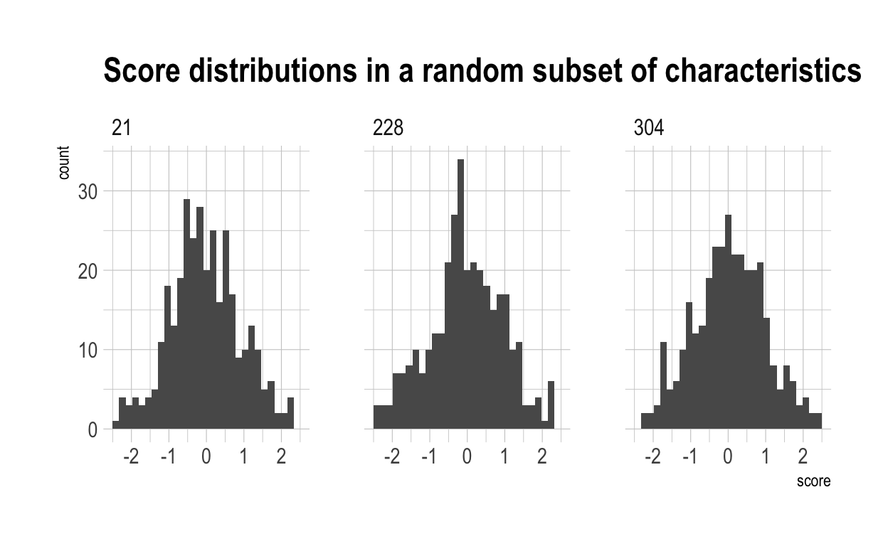
First, I create 1000 individuals. For each of those individuals, I then compute a random score for each of the 500 characteristics, following a normal distribution. Those scores range from (approximately) -3 to (approximately) 3, with a mean at 0 and a standard deviation of 1.
characteristics <- expand.grid(individual = 1:n_individuals,
                               characteristic = 1:n_characteristics)
characteristics$score <- rnorm(n_individuals * n_characteristics)
Here’s a random sample of the individual/characteristic pairs created by that code, together with the randomly-generated scores.
| individual | characteristic | score |
|---|---|---|
| 342 | 471 | 0.1297448 |
| 476 | 348 | 0.6015418 |
| 38 | 66 | -0.0434303 |
| 915 | 464 | 0.0314398 |
| 591 | 306 | 0.8712442 |
This graph shows the distribution of scores in a random subset of characteristics, as created by the above proccess.
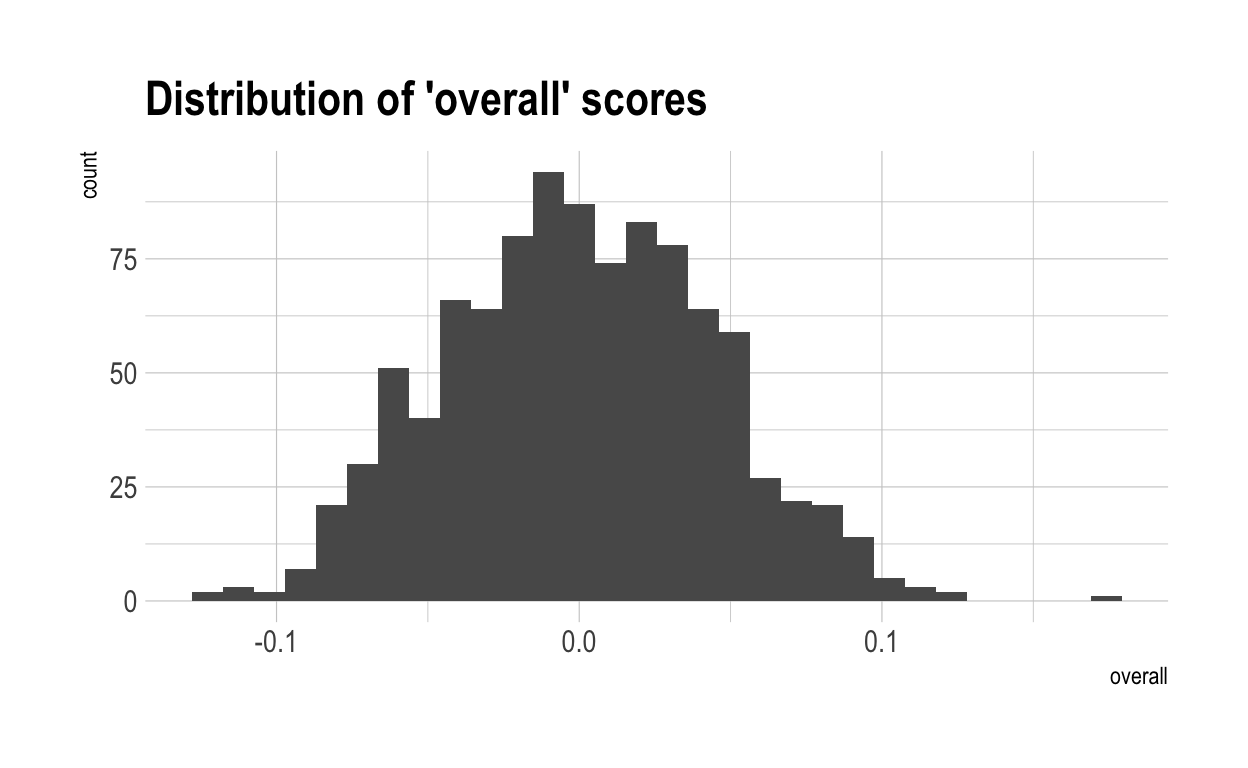
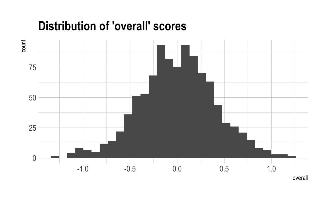
Now, I have computed a “overall” score for each individual. This is simply each individual’s average score accross all 500 characteristics. Because each of the characteristics is independent from each other, they will typically cancel each other out. The chances of someone scoring highly in many characteristics are low. This generates a much tighter distribution for ‘overalls’. This is shown below.
by_individual <- characteristics %>%
  group_by(individual) %>%
  summarise(overall = mean(score))
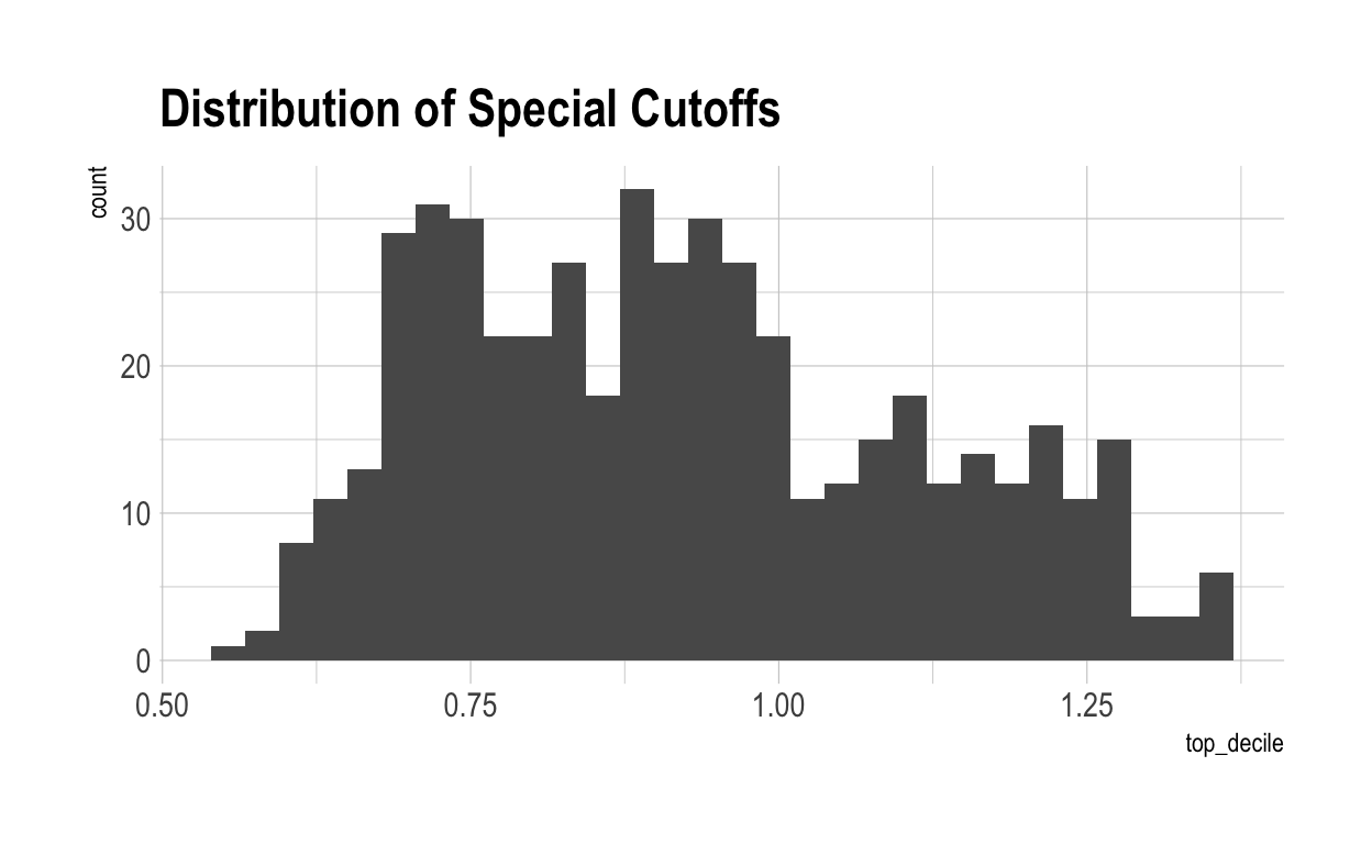
Now let’s work out what score you have to get to be special in each characteristic. This can be done mathematically, of course, but let’s do it using the simulated data. Here’s the distribution for top-10% cut-off points:
cutoffs <- characteristics %>%
            group_by(characteristic) %>%
            summarise(top_decile = quantile(score, 0.9))
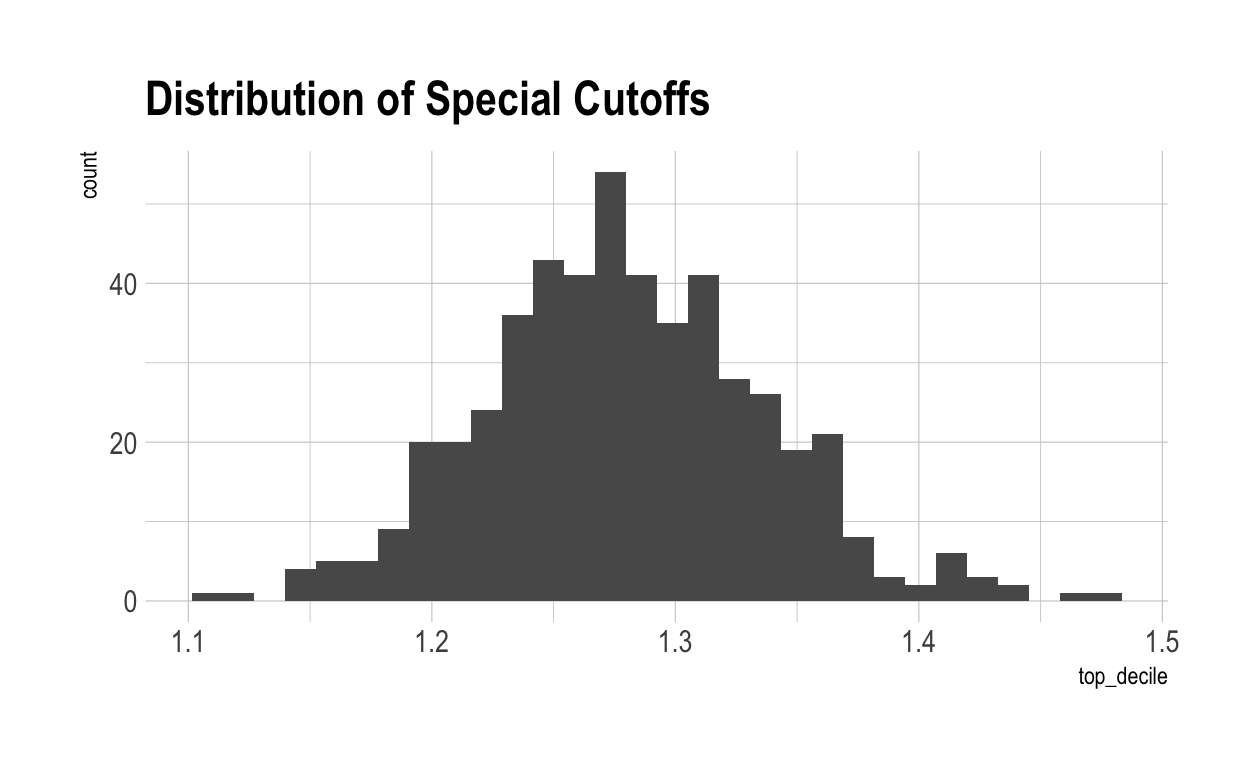
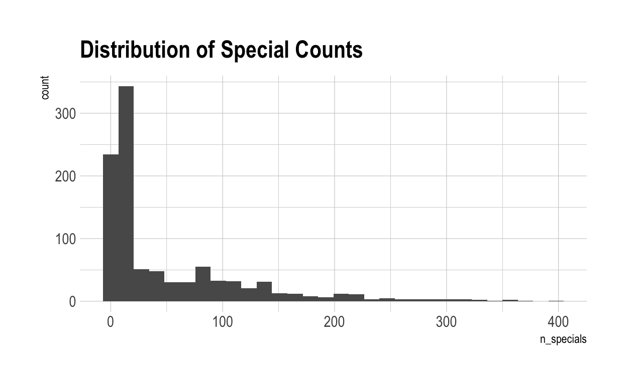
As you can see, on average, individuals have to have a score greater than 1.28 to be considered ‘special’ in that characteristic. Now, let’s see how special each individual is – measured by the number of scores above the special cut-off for that characteristic they achieve.
special_count <- characteristics %>%
                    inner_join(cutoffs) %>%
                    mutate(special = score >= top_decile) %>%
                    group_by(individual) %>%
                    summarise(n_specials = sum(special)) %>%
                    arrange(n_specials)
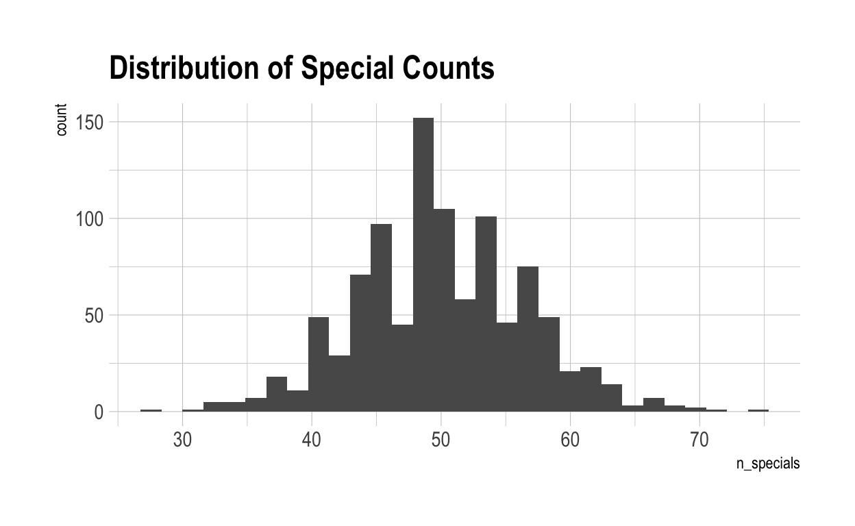
Overall, there are 0 individuals who are not special in anything.
A Slightly More Realistic Model
Obviously it is not true that each of these characteristics is unrelated to each other. For instance, someone who is good at breast stroke swimming would also probably be better at rowing than someone who can’t swim at all. Let’s introduce some interpendence.
In this model, I introduce four ‘meta-characteristics’ which could impact all other characteristics. These four meta-characteristics have nothing special about them – and there could in fact be an arbitrary number of meta-characteristics. But, for the sake of this argument, let’s assume there are four meta-characteristics. These meta-characteristics impact every other characteristic, but are indepdent from each other. Let’s call them intelligence (I), creativity (C), emotional capability (E), and physical aptitude (P). (Again, these four are just picked out of thin air. What they are doesn’t really matter.) Obviously, not every characteristic will depend equally on those four. Some skills – like chess – might mostly be based on I, while others – like sprinting – might depend mostly on P. Moreover, not all the variation in skills will be due to those four. Each skill might itself have something unique about it – let’s call it U. Let’s say each of those factors contributes \(x\)% to an individual’s total skill in each pursuit. Their total score could be given by
\[ T = x_II+x_CC + x_EE + x_PP + x_uU \] Necesarily, \(x_I+x_C+ x_E+ x_P+ x_u=1\).
Now, let’s randomly generate 500 non-meta characteristics, each with their own \(x\)-values.
characteristics_to_generate <- 500

generate_coefficients <- function() {

  coefs <- numeric(5)

  # Ensures that the coefficients all add up to 1
  remaining_pct <- 1
  for (i in 1:4) {
    coefs[i] <-runif(1, max=remaining_pct)
    remaining_pct <-remaining_pct-coefs[i]
  }
  coefs[5] <- remaining_pct

  match <- as.data.frame(sample(coefs))
  match$code <- c('I','C','E','P','U')

  to_return <- match %>% pivot_wider(names_from = code, values_from = "sample(coefs)")

  return(as.data.frame(to_return))

}

meta.coefs <- data.frame(characteristic=numeric(),
                      I=numeric(),
                      C=numeric(),
                      E=numeric(),
                      P=numeric(),
                      U=numeric())

for (i in 1:characteristics_to_generate) {
  d <- generate_coefficients()
  d$characteristic <- i
  meta.coefs <- meta.coefs %>% bind_rows(d)
}
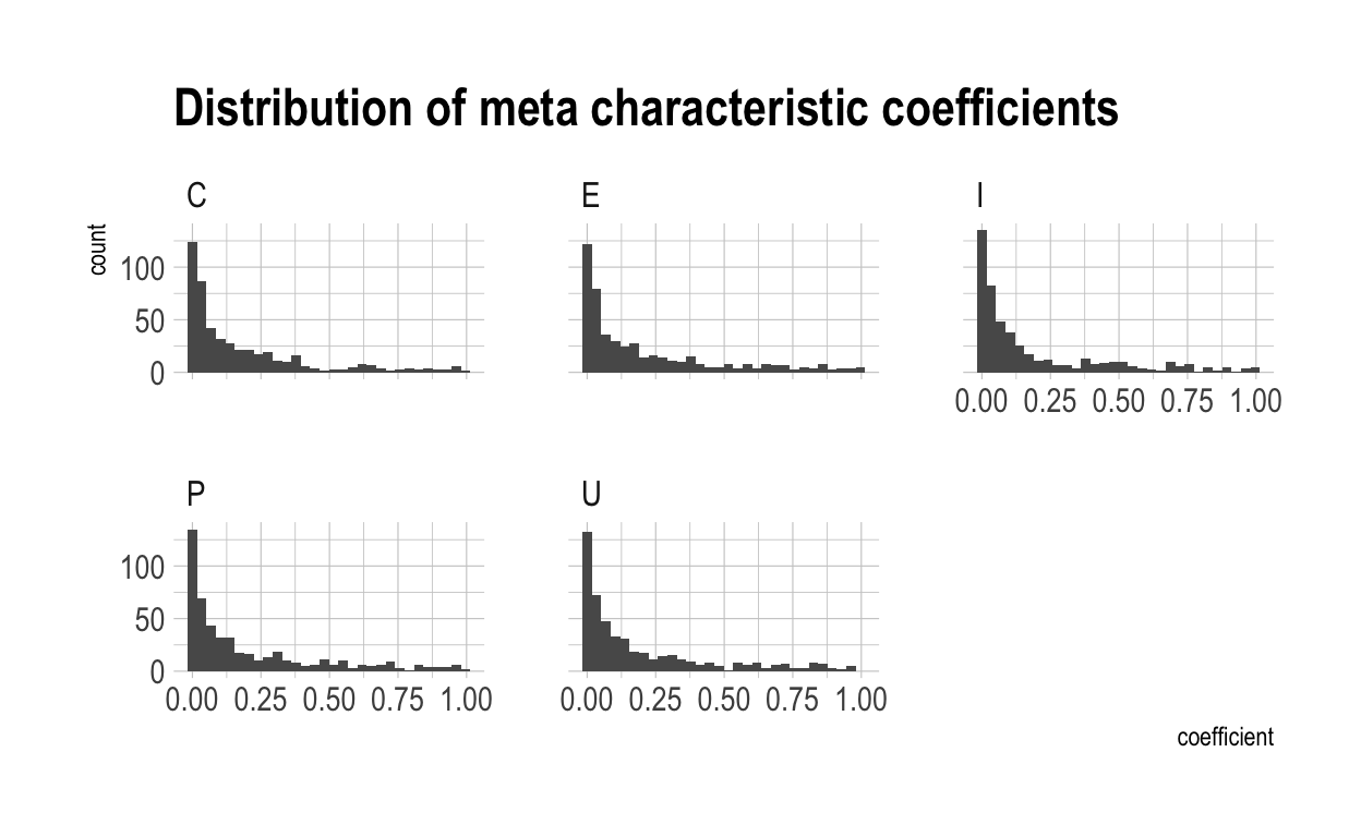
Here’s what a sample of those non-meta characteristics, together with their randomly-generated coefficients, looks like:
| characteristic | I | C | E | P | U |
|---|---|---|---|---|---|
| 420 | 0.0788430 | 0.1893252 | 0.0203186 | 0.0117644 | 0.6997489 |
| 263 | 0.1120078 | 0.2809451 | 0.0302990 | 0.0806747 | 0.4960733 |
| 394 | 0.7091299 | 0.2013960 | 0.0071228 | 0.0790491 | 0.0033022 |
| 438 | 0.0003763 | 0.0058852 | 0.9916222 | 0.0020564 | 0.0000599 |
| 153 | 0.6192793 | 0.1214425 | 0.2363449 | 0.0086217 | 0.0143115 |
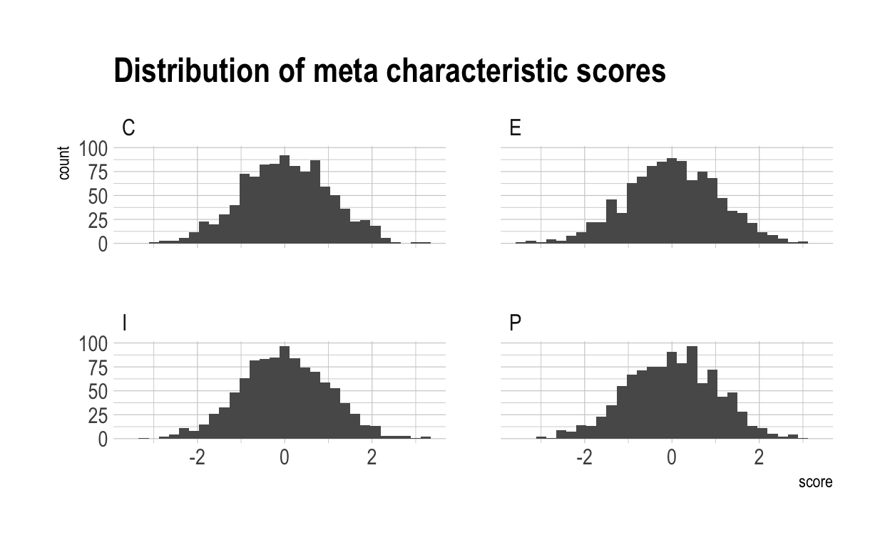
Now we have to generate the meta-characteristic scores for each individual. Once again, these will normally distributed.
meta.indiv <- data.frame(individual=1:n_individuals,
                      I=rnorm(n_individuals),
                      C=rnorm(n_individuals),
                      E=rnorm(n_individuals),
                      P=rnorm(n_individuals))
Here’s what a sample of these randomly-generated scores looks like:
| individual | I | C | E | P |
|---|---|---|---|---|
| 880 | 0.1699370 | -0.4522160 | 0.2598345 | -0.7248564 |
| 733 | -2.6323271 | -1.0038183 | -0.7816725 | 0.1492215 |
| 884 | -1.2243767 | -0.1290599 | 0.6870071 | 0.5120966 |
| 807 | -1.6953239 | 2.1782578 | -0.2234895 | -0.6952718 |
| 477 | 0.9212673 | 1.2377749 | -0.9057107 | -0.7111390 |
This is what the distribution of meta scores looks like over the whole population:
Now we have to combine these two to create the characteristic scores for each individual in the normal (non-meta) characteristics. Further, we have to generate the unqiue terms for each individual/characteristic pair representing the individual’s score in that particular characteristic which is indepedent of the meta-characteristics.
nonmeta.indiv <- expand.grid(individual = 1:n_individuals,
                             characteristic = 1:characteristics_to_generate)
nonmeta.indiv$U <- rnorm(n_individuals*characteristics_to_generate)

nonmeta.indiv <- nonmeta.indiv %>%
  inner_join(meta.indiv) %>%
  inner_join(meta.coefs,
             by=c("characteristic"),
             suffix=c(".indiv", ".coef")) %>%
  mutate(score = (I.indiv * I.coef) + (C.indiv * C.coef) +
           (E.indiv * E.coef) + (P.indiv * P.coef)  +
           (U.indiv * U.coef))
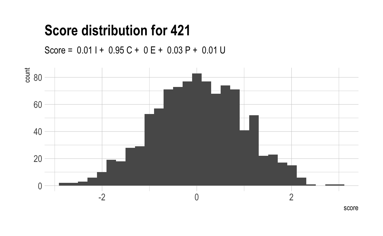
Here’s what a sample of these individual/characteristic pairs looks like:
| individual | characteristic | U.indiv | I.indiv | C.indiv | E.indiv | P.indiv | I.coef | C.coef | E.coef | P.coef | U.coef | score |
|---|---|---|---|---|---|---|---|---|---|---|---|---|
| 842 | 25 | -0.11 | -0.82 | 0.32 | -0.57 | 0.90 | 0.84 | 0.12 | 0.02 | 0.00 | 0.02 | -0.66 |
| 793 | 151 | 0.37 | 0.61 | 0.13 | -0.01 | 0.53 | 0.52 | 0.04 | 0.41 | 0.01 | 0.02 | 0.33 |
| 211 | 481 | -0.31 | 1.26 | -0.73 | -0.15 | -0.83 | 0.53 | 0.00 | 0.00 | 0.03 | 0.43 | 0.52 |
| 948 | 393 | 1.15 | -0.24 | 1.22 | 0.56 | 0.11 | 0.23 | 0.13 | 0.06 | 0.52 | 0.06 | 0.27 |
| 764 | 331 | -0.45 | 2.18 | 0.46 | 0.72 | 0.07 | 0.09 | 0.04 | 0.19 | 0.03 | 0.65 | 0.07 |
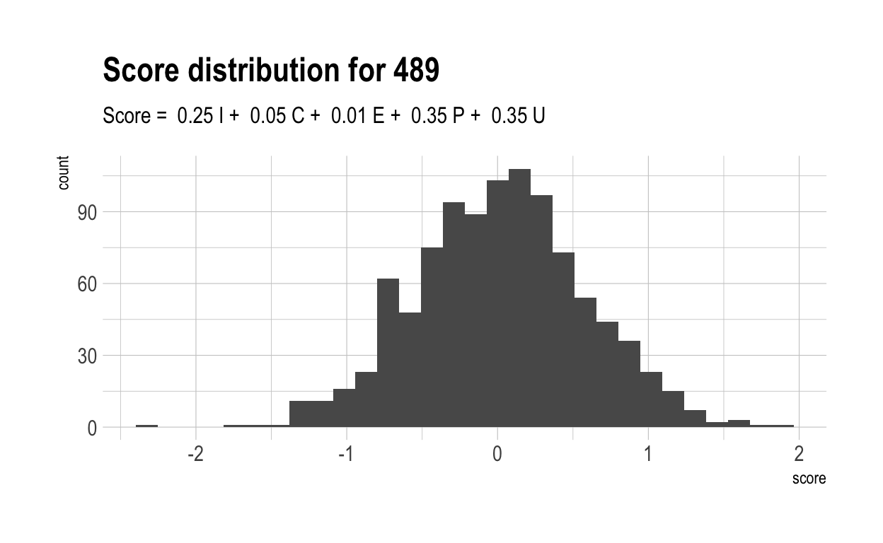
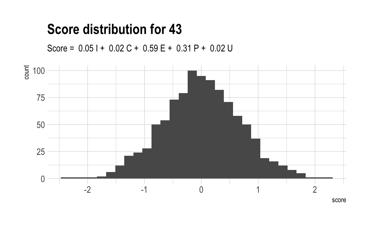
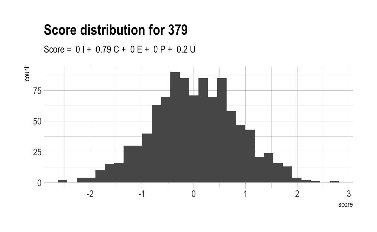
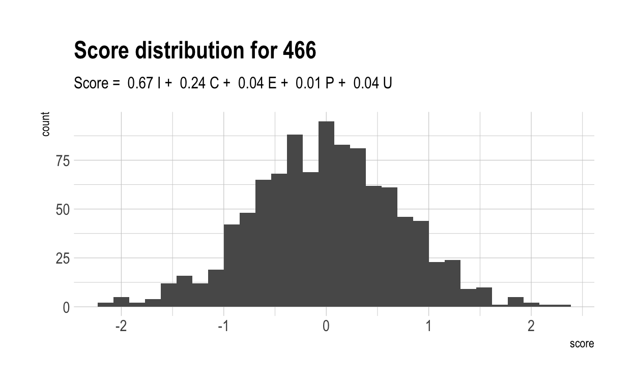
Here are the distributions of those scores for 5 randomly chosen characteristics, together with their score formulae.
Now, let’s once again compute a “overall” score for each individual. Naturally, these have a much wider range than did overall scores in the previous, more naive model. This is because much of the variance in overall score is driven by only 4 variables. With only 4 variables, there are likely to be many more people who cannot make up their diffencies with strong performances elsewhere.
by_individual2 <- nonmeta.indiv %>% group_by(individual) %>% summarise(overall = mean(score))
Now let’s work out what score you have to get to be special in each characteristic. Naturally, because of the broader dispersion of outcomes shown above, the score to become special is lower in a world where skills are inter-related.
cutoffs2 <- nonmeta.indiv %>%
            group_by(characteristic) %>%
            summarise(top_decile = quantile(score, 0.9))
Then let’s apply those requirements to all of the individual scores in each characteristic. Once again, because of the dispersion in outcomes, we see a very different graph.
special_count2 <- nonmeta.indiv %>%
                    inner_join(cutoffs2) %>%
                    mutate(special = score >= top_decile) %>%
                    group_by(individual) %>%
                    summarise(n_specials = sum(special)) %>%
                    arrange(n_specials)
In this new model, 4 individuals are not special in anything.
Conclusions
On slightly more realistic assumptions, therefore, it looks like not everyone is guaranteed to be special. However, the different results we recieved from each model are important in themselves. When more of one’s variance is due to a few factors, that increases the likelihood that people will not be able to compensate for weakness in one area with strength in another. That has interesting implications for how we think about, for instance, the disappearance of manual labour work. As jobs become increasing knowledge-focused, our performance coalesces more and more around one factor – intelligence. That increases the likelihood that some people will fall behind, even if, in previous times, their physical strength or other characteristics could have compensated. We should be careful to consider this when designing social policy.